


Abstract
In the event of a potentially catastrophic asteroid impact, with sufficient warning time, deploying a nuclear device remains a powerful option for planetary defense if a kinetic impactor or other means of deflection proves insufficient. Predicting the effectiveness of a potential nuclear deflection or disruption mission depends on accurate multiphysics simulations of the device's X-ray energy deposition into the asteroid and the resulting material ablation. The relevant physics in these simulations span many orders of magnitude, require a variety of different complex physics packages, and are computationally expensive. Having an efficient and accurate way of modeling this system is necessary for exploring a mission's sensitivity to the asteroid's range of physical properties. To expedite future simulations, we present a completed X-ray energy deposition model developed using the radiation-hydrodynamics code Kull that can be used to initiate a nuclear mitigation mission calculation. The model spans a wide variety of possible mission initial conditions: four different asteroid-like materials at a range of porosities, two different source spectra, and a broad range of radiation fluences, source durations, and angles of incidence. Using blowoff momentum as the primary metric, the model-initiated simulation results match the full radiation-hydrodynamics results to within 10%.
Export citation and abstract BibTeX RIS

Original content from this work may be used under the terms of the Creative Commons Attribution 4.0 licence. Any further distribution of this work must maintain attribution to the author(s) and the title of the work, journal citation and DOI.
1. Introduction
It is estimated that approximately 5000 metric tons of space debris collide with the Earth every year, mostly in the form of harmless dust particles (Rojas et al. 2021). By extension, collisions with larger objects in the solar system, such as an asteroid, also occur regularly. These events, though rare, can cause extensive destruction on a regional to global scale, depending on the amount of energy released. However, with sufficient preparation and warning time, an impact from a small solar system object is one natural disaster that can be completely averted with modern technology. To this end, a global campaign collectively known as "Planetary Defense" is well underway to locate objects that pass close to Earth's orbit, or near-Earth objects (NEOs) 1 ; develop mitigation strategies for potential impactors; and, for unavoidable collisions, assess the consequences for emergency response (National Research Council 2010). Specifically, in the United States, the Planetary Defense Coordination Office was established in 2016 (Landis & Johnson 2019) to oversee many growing efforts across various agencies and later help implement the National Near-Earth Object Preparedness Strategy and Action Plan (NSTC 2018, 2023).
To ensure that potentially hazardous objects are located before they become a threat, the George E. Brown Jr. Near-Earth Object Survey Act of 2005 (U.S. House. 109th Congress, 1st Session 2005) mandated that NASA locate 90% of NEOs larger than 140 m across, which could cause regional devastation large enough to warrant an attempted mitigation mission, by 2020. As of 2021, it was estimated that only ∼50% of such NEOs had been found (Harris & Chodas 2021). Though the eventual launch of the NEO Surveyor mission will accelerate the process (Grav et al. 2021), completing the mandate will not eliminate all of the risk. Asteroids that are either slow-moving (Wainscoat et al. 2022) or small in size (<140 m) will remain serious challenges for early detection systems. Small asteroids in particular present complications; as the NEO diameter decreases, both the population size and detection difficulty increase. Impacts from small asteroids can also cause substantial damage, as seen in the two most recently recorded impacts. The first, in Tunguska, Russia (year: 1908, size: ∼55 m, a once per 100–1000 yr event; Napier & Asher 2009), flattened 2000 km2 of forest, and the second, more recently, in Chelyabinsk, Russia (year: 2013, size: ∼19 m, a once per 20–100 yr event; Brown et al. 2013; Harris & Chodas 2021), injured over a thousand people and damaged several thousand buildings.
In the case of mitigation missions, substantial progress has been achieved in developing options for preventing impacts (Dearborn & Miller 2015), most notably culminating in NASA's Double Asteroid Redirection Test (DART), which executed the first successful deflection of an asteroid in 2022 (Thomas et al. 2023). The DART mission impacted the smaller of a binary asteroid pair to demonstrate a kinetic impact deflection, which, for conditions when it can be effective, is considered the preferred mitigation mission option (National Research Council 2010). However, while the limits of kinetic impactor effectiveness depend upon the individual orbital and geotechnical characteristics of each asteroid (Barbee et al. 2018; Dearborn et al. 2020), the likely applicable size range (∼100–200 m for a rubble-pile asteroid) and warning time constraints (≳10 yr) are restrictive. For example, with a maximum-mass Falcon Heavy payload (4500 kg) intercepting an asteroid at 6 km s−1 (DART velocity), a 170 m diameter spherical asteroid with a bulk density of 2 g cc−1 would have a deflection velocity (Δv) of 1.05 cm s−1. Applying the nominal Earth-miss condition defined in Ahrens & Harris (1992), Δv = 10 cm s−1 per year of warning time, this intercept would need to occur approximately 10 yr or more before the Earth impact date. As described in Dearborn & Miller (2015), kinetic impactor effectiveness is also limited by the maximum velocity that can be delivered to an asteroid without unintentionally weakly disrupting it. This limit, sometimes provided as a percentage of asteroid escape velocity, may depend upon characteristics such as porosity, strength, and rotational state but generally becomes easier to exceed with smaller asteroid sizes. If a kinetic impactor mission design requires the deflection velocity to be either greater than the disruption limit or what can be delivered by available launch capabilities, a longer warning time would be necessary or an alternative mission type should be considered.
Utilizing a nuclear explosive device (NED) to carry out a mitigation mission is a versatile, effective approach to deflecting or disrupting NEOs, including more challenging scenarios. An NED has the highest energy output per unit mass that modern technology can produce. Yield delivered to a potential NEO can be tuned postlaunch by adjusting the height of burst (HOB) between the device and the object's surface. If the mission design requires that the NEO be kept intact and merely given a "push" (a deflection mission), the nuclear device can be detonated at a large HOB compared to the NEO diameter. The radiation from the detonation will propagate freely through the vacuum of space to illuminate a large swath of the object's surface area, causing the material to heat up, vaporize, and expand rapidly. The "blowoff momentum" (pb ) of the newly ejected mass is balanced by an equal momentum in the opposite direction that alters the NEO's total velocity. If the NEO is too small to withstand an attempted deflection mission, or if the warning time requires an impulse so aggressive that it risks fragmenting the object into several potential impactors, the NED can be detonated in close proximity to the object for an intentional disruption mission. In addition to the substantial vaporized ejecta, a successful disruption will cause a shock wave to propagate through the asteroid, breaking it into many small, harmless, fast-moving fragments. Simulations have shown that if such a mission is carried out at least a month before impact, for a 1 Mt device detonated 15 m from a 100 m asteroid, over 90% of the NEO's material will miss the Earth entirely (King et al. 2021). However, if such a mission were attempted via a flyby spacecraft, fast closing speeds (∼10 km s–1) and radar functionality would limit standoff distance precision to the tens of meters range. A slower closing velocity or future radar developments will improve the capabilities of a flyby mission. For a mission design that either requires a precise, small (tens of meters) standoff distance or deploys multiple sequential device detonations from a single spacecraft, a full rendezvous mission will be required. In either case, the detonation is conducted millions of miles from Earth, where the device's radiation does not pose a threat. 2
A growing campaign to fully simulate nuclear mitigation missions has been progressing over the past couple decades (Dearborn 2004; Dearborn et al. 2007, 2020), though the problem presents significant modeling challenges. Even when an asteroid's complex structure and inhomogeneous material properties are set aside and the object is approximated as a uniform sphere, the sheer breadth of the required physics presents difficulties. When the radiation from the NED first penetrates the surface of the asteroid and deposits energy, the length and timescales that must be resolved are on the order of micrometers and nanoseconds, respectively. Fully simulating the energy deposition requires particle transport within a full radiation-hydrodynamics code equipped with detailed material models and is very computationally expensive, since the time steps must be small to model the interaction of the radiation with the asteroid. It can take weeks to run a simulation even on 200–300 CPUs. Eventually, when the energy has propagated deeply enough to form a shock wave, the length and timescales could span tens to hundreds of meters and seconds to minutes, depending on the nature of the mission. For this stage, having accurate damage and strength models to inform the breakup process would be ideal. No single code can encompass all 10 orders of magnitude while correctly accounting for all of the different physics packages, so dividing the problem into stages and handing off the progression to codes that cover the relevant physics of the next stage is desirable.
This code-to-code handoff method works well for the case of neutron radiation from an NED, where the energy is almost instantly deposited compared to hydrodynamic motion, and the deposition depth is larger compared to the other forms of radiation output. Using energy deposition profiles calculated with a Monte Carlo N-Particle transport code (MCNP, developed by LANL; Pelowitz et al. 2005) from neutrons with energies often seen in common fission and fusion reactions, studies showing the limits and effectiveness of NED neutrons were successfully carried out by Bruck Syal et al. (2013) and Horan et al. (2021), respectively. However, based on Glasstone Sections 1.26, 1.77, and 8.03 and Table 10.138 (Glasstone & Dolan 1977), neutrons only make up approximately 1% of the prompt energy output from an NED. 3 Instead, the vast majority of the energy (∼70%) is carried by soft X-rays, with gamma rays (∼0.3%) and kinetic energy from debris (∼28%) making up the remainder. Thus, having a working model that encompasses the energy deposition of the X-ray radiation represents the highest priority in terms of radiation sources for nuclear mitigation missions. To address this need, Howley et al. (2014) and Managan et al. (2015) proposed an analytical model based on the Beer–Lambert law, where the penetration depth and energy coupling efficiency for the X-ray energy/material combination of interest were determined using MCNP and Mercury (a Monte Carlo particle transport code based at LLNL; Brantley et al. 2012). The analytical model consisted of a simple summed exponential function that could be tailored based on the energy fluence arriving at the asteroid's surface, as well as the angle of incidence. Due to the functional dependence on the angle of incidence, this model could easily be implemented into a realistic asteroid shape model, which was successfully achieved in Herbold et al. (2015), Owen et al. (2015), and King et al. (2021).
Unfortunately, in MCNP and Mercury, all photons are approximated as gamma rays, so the nuclear reactions that are tracked by the simulation do not take into account the relevant atomic processes that happen when X-rays interact with and heat the matter, which require a full radiation-hydrodynamics code equipped with detailed equation-of-state (EOS) data to model, such as in Dearborn et al. (2020). As the X-rays heat the material, some energy is reradiated back into space, and the ability of the material to absorb the energy from the photons (opacity) changes over the duration of the illumination in response to the radiation that has already arrived. Both processes are significant enough that neither the unaltered summed exponential nor one scaled down by the energy fraction lost to reradiation can accurately reproduce the amount of blowoff momentum produced by a full rad-hydro simulation. In principle, it is possible to continue using an exponential energy deposition with a path length calibrated to the melt depth (Howley et al. 2014). However, the technique begins to fail at the high-fluence ranges (>0.04 kt m−2) required for disruption, where a developing thermal wave alters the resulting blowoff momentum. Even at low-fluence ranges, the exponential function requires extremely fine surface resolution to resolve properly, which further exacerbates the already-challenging simulation setup. For these reasons, the exponential energy deposition was set aside in favor of using results taken directly from a full radiation-hydrodynamics simulation. Previous studies covered cases that did not reach the high-fluence regime and assumed that the effects on the blowoff momentum resulting from the evolving material opacities would not be significant. This study represents the first exploration of NED energy deposition utilizing a full rad-hydro simulation equipped with evolving opacities, which also enabled it to be the first comprehensive effort to explore the high-fluence regime where a disruption-style mitigation mission would operate.
This paper presents a completed energy deposition model for initializing hydrodynamic simulations of nuclear mitigation missions for the purposes of planetary defense. The model encompasses four common materials found in NEOs and fluence ranges that cover realistic deflection and disruption scenarios. The generated energy deposition functions take into account angle of incidence, porosity, reradiation, reflected photons, and all other relevant physics processes so that no other input information is required. The subsequent sections in this paper will cover the development of the model and how to implement it and then compare the results between model-initiated hydrodynamic simulations and their analogous full rad-hydro calculations for the purpose of quantifying uncertainties. The creation of this simplified energy deposition framework represents a significant advancement in the realm of simulating nuclear mitigation missions with accuracy. It paves the way for both detailed simulations of specific NEO missions and larger sensitivity studies based on a potential impactor's many unknown physical properties (shape, structure, rotation, material, density, even size) to be performed more easily before a crisis arises. The findings from the sensitivity analyses would help quickly inform decision-makers what ranges of potential asteroid properties a mission would likely be successful in mitigating, depending on how much is known about the incoming NEO. Simulation studies such as these are prioritized in Goal 2 of the National Near-Earth Object Preparedness Strategy and Action Plan (NSTC 2023) and further emphasized in the recent Planetary Science and Astrobiology Decadal Survey (National Academies of Sciences, Engineering, and Medicine 2022).
The python scripts for implementing the energy deposition model in a hydrodynamic simulation and supporting data used to inform the model can be downloaded from the Burkey & Managan (2023) repository on GitHub.
2. Simulation Setup
2.1. Scope of Study
The energy deposition model described in this paper strives to encompass as many realistic scenarios as possible spanned by the relevant parameters listed below.
Materials—Silicon dioxide (SiO2), forsterite (Mg2SiO4), ice (H2O), and iron (Fe) were chosen to represent the NEO materials. Though a potential impactor's composition would be much more complex, the materials listed are common components of more intricate minerals and expected to behave similarly. Bulk densities of asteroids with diameters less than 50 km (of interest for mitigation missions) are clustered in the 1–3 g cm−3 range. These can be reasonably well represented with our set of materials by including either macro- or microporosity (or a combination; Carry 2012). For deflection simulations, previous work by Dearborn et al. (2020) has shown that final velocities are relatively insensitive to minor differences in the type of silicate EOS used (e.g., using hydrated forsterite produced similar outcomes to SiO2). The largest compositional lever on deflection outcomes is the atomic mass of the elements, which controls the X-ray energy deposition length scale. For this reason, we choose materials that are reasonable low-Z (H2O, ice) and high-Z (Fe) end-members for materials present at asteroid or comet surfaces, along with two mid-Z rocky materials (SiO2 and Mg2SiO4). Each selected material has well-established EOS data to inform the radiation transport simulations.
Porosity—The energy deposition model was developed using simulations with microporosities (ϕ) ranging from 0% to 80% for all materials, which covers the vast majority of possible NEOs. Extrapolation to higher porosity is possible but should be attempted with caution. Larger macroporosity features are better suited for full-scale hydrodynamic models and are excluded to keep the size and scope of the study manageable.
X-ray source spectrum—The NED thermal radiation can be approximated by a blackbody (BB) source with a peak at ∼4 keV according to Sections 7.73 and 7.79 of Glasstone & Dolan (1977). For simplicity and to provide multiple options, the NED sources we simulate are approximated as 1 and 2 keV BBs with spectra pictured in Figure 1 and peaks at ∼2.8 and ∼5.6 keV, respectively.

Figure 1. Normalized 1 and 2 keV BB spectra.
Download figure:
Standard image High-resolution imageX-ray source strength—The X-ray fluences (f) that were modeled range from 10−4 to 1 kt m−2. The lowest value represents a small surface layer melt, which is well suited for the edges of illumination in a deflection mission. The highest point in the fluence range roughly corresponds to the energy per area seen by the closest point of an NEO when a 1 Mt NED is detonated 10 m from the surface, a realistic disruption scenario.
Source duration—The NED's radiation is released over a length of time (tend) that depends on the number of neutron generations it takes to deliver the device's yield. The fast neutron generation time in fission is approximately 0.01 μs or 10 ns. Section 1.57 of Glasstone & Dolan (1977) sets a lower limit of the NED source duration as ∼10 ns (the last e-folding of the energy production) and estimates that the vast majority of the yield in a 100 kt device would be released within 70 ns. To encompass a broad range of scenarios, NED sources ranging between 10 and 100 ns were modeled and included in the deposition formulation. All of the sources were approximated as constant/having no time dependency, though uncertainties arising from this assumption are explored at the end of the paper.
To keep the scope of this study manageable and not introduce additional layers of complexity, all test asteroids simulated in this study will be homogeneous spheres. Additional features such as macroscopic variation in properties and irregular shapes will be the subject of future work and are discussed in Section 6.
2.2. Simulation Codes
The radiation-hydrodynamics code selected to simulate the process of X-rays impinging on an NEO surface was the Kull multiphysics code (Rathkopf et al. 2000). Developed at LLNL primarily for simulating inertial confinement fusion processes at the National Ignition Facility, the code is multidimensional, mesh-based, and able to accommodate many types of physics, including multiple radiation transport options: diffusion, discrete ordinates (also known as SN ), and implicit Monte Carlo (IMC).
Of the three, IMC was selected as the transport package of choice for the simulations described in this study. This was done because the simulation has an angularly homogeneous point source of radiation situated in a vacuum. The diffusion approximation loses all angular information about the direction of radiation propagation and calculates the radiation flux via Fick's law using a diffusivity proportional to the inverse of the opacity. Diffusion thus has particularly large errors when simulating radiation in a vacuum and would deposit energy even in the shadowed part of the asteroid. The SN method computes the propagation of radiation along specific directions chosen during problem setup; these specific directions are called discrete ordinates in the nomenclature of the method. In nonopaque materials, the radiation propagating in the specific directions will diverge as they move away from a point source, leaving regions of anomalously low radiation intensity between them. This discretization error is known as a "ray effect." The ray effects introduced by SN transport would have created nonsmooth energy deposition on the asteroid surface because in a vacuum, ray effects are not reduced by absorption or scattering (Castor 2004).
Since it was designed for high-density and high-energy conditions, Kull would occasionally have difficulty simulating expanding, low-density material, such as would be required in a nuclear mitigation mission. In some instances, depending on the EOS data, Kull would pull the material into tension, which decreased the simulated blowoff momentum in an unrealistic manner. For those cases, the Kull simulation could be handed off to a similar mesh-based hydrodynamic code better suited for the conditions, before tension arose, in order to complete the full simulation with integrity. The handoff code, Ares (Darlington & McAbee 2001; Bender et al. 2021), was also used for comparison and cross-checking pure hydrodynamic runs initialized with the energy deposition model.
For Kull simulations where porosity was nonzero, a simple snowplow model 4 was used to simulate the material's behavior under compression. Ares utilized a more sophisticated model that lowers porosity when the pressure is above a corresponding crush curve pressure, but a similar snowplow model was also implemented for cross-code comparison. There were no distinguishable differences in the Ares results between the two porosity models, which lends confidence to the effectiveness of the snowplow model in this scenario.
2.2.1. EOSs and Initial Conditions
To accurately account for each material's thermodynamic properties during the heating process, a tabular EOS containing information on the pressure, specific internal energy, sound speed, etc. for a grid of density and temperature points was utilized for each material. The SiO2 and Mg2SiO4 EOSs were constructed using M-ANEOS (Thompson & Lauson 1974; Melosh 2007; Thompson et al. 2019). The SiO2 table uses the parameters from Melosh (2007), and the Mg2SiO4 table is from Stewart et al. (2020). M-ANEOS accounts for the molecular clusters that appear in the vapor phase and uses a potential for the expanded-solid state that better describes these geologic materials. The EOSs for water and iron were constructed using an approach similar to the QEOS framework of More et al. (1988) but including some additional features from Young & Corey (1995). These EOS tables are available in the aforementioned GitHub repository (Burkey & Managan 2023).
Each material is initialized to the EOS-determined reference density, ρ0, and initial temperature (shown in Table 1), so the simulation starts with zero pressure. For porous materials, this means that the density of the matrix material equals the reference density or that the bulk density is ρ = ρ0(1 − ϕ). This is done to prevent any motion from tension or positive initial pressures, which could compete with the blowoff momentum effects. Both simulations used a multigroup radiation model with 200 groups spaced logarithmically from 0.003 to 2000 keV. The opacities are averaged within each group.
Table 1. Initial Conditions for Each Material (Reference Density and Temperature)
| SiO2 | Mg2SiO4 | Fe | H2O | |
|---|---|---|---|---|
| ρ0 (g cm–3 ) | 2.65 | 3.22 | 7.877 | 1.0 |
| T (K) | 298 | 298 | 200 | 200 |
Note. Each combination of values was selected to ensure the initial pressure was set to near 0 and the system was without tension. The temperatures listed are for setups with zero porosity; setups with nonzero porosity used initial temperatures of 200 K since the porosity model zeros the pressure.
Download table as: ASCIITypeset image
2.3. Geometrical Setup and Meshing
The full, 2D geometrical setup of our simulations with all relevant variables can be found in Figure 2. Because the problem is cylindrically symmetric around the axis connecting the NED source and the center of the NEO, a 3D approximation can be achieved by rotating around the same axis. The NEO 2D mesh was constructed using a number of equally spaced wedges fanning out from the θ = 0 axis. The number of required wedges would vary based on the HOB and the simulation being used. The wedges would then be radially segmented into ratioed zones based on the specified (very small) thickness of the surface zone and the zone count. The number of required zones depended on the code used, the material-opacity combination, and the flux of energy arriving from the source.
Figure 2. Geometric setup of deflection simulations. All NEOs are approximated as homogeneous spheres with radius R. The distance between the closest NEO surface point and the NED (represented as a point source) is the HOB. The cone of radiation illuminates angles θ = 0 to  of the NEO's surface, with the radiation angles of incidence β ranging between 0◦ and 90◦. Hereafter, β will be converted to
  for simplicity. The distance between the NED and an illuminated point on the NEO's surface is denoted as S.
Download figure:
Standard image High-resolution imageA 1D simulation setup is similar to a single wedge in the 2D geometrical setup, except the wedge shape is exchanged for a 1 cm2 column. The ratioed radial zoning is kept the same, and the end of the mesh is cut off between 10 and 100 cm, depending on how far the energy propagates in the given simulation time, rather than a column length equal to R. The β between the NED radiation and NEO surface is also preserved.
For every mesh parameter, a 1D resolution study was performed based on material and NED fluence level to ensure the accuracy of the results to within a few percent. Each study involves running a suite of simulations with a varying mesh parameter to determine a resolution value where the result converges. Though the number of zones in each direction matters, the most sensitive parameter was the thickness of the surface zone. Results from a suite of 1D IMC simulations at normal incidence for each material at a range of fluences can be seen in Figure 3, which convey when the surface zone thickness converges in each case. The results were drawn from cases using a 1 keV BB spectrum, a source duration of 10 ns, and zero porosity. For a 2 keV BB or nonzero porosity, the required zone thickness would be slightly coarser, while a longer source duration would require slightly finer resolution. All simulations were run with a surface thickness resolution smaller than would be required for convergence.

Figure 3. Resolution study of a 1D simulation suite measuring blowoff momentum and parsed by material and fluence. The varied mesh parameter is the thickness of the first zone, which was by far the most sensitive mesh-constructing value.
Download figure:
Standard image High-resolution image3. Model Development
The energy deposition model's foundation is comprised of several large suites of energy density profiles taken from radiation transport simulations in Kull at a time shortly after the source has finished illuminating the surface but before substantial hydrodynamic motion occurs. This section outlines the construction of the model, beginning with the time when the energy deposition profile snapshot is taken, comparing 1D results to 2D results to ensure consistency, and then building each layer of the model by fitting suites of deposition profiles to a functional form.
3.1. Blowoff Momentum
As previously discussed, the primary metric used in this study for comparison between simulations is the amount of momentum carried by the mass ejected from the surface of the asteroid: the blowoff momentum, or pb . By Newton's third law of motion, the blowoff momentum is closely coupled to the momentum imparted to the full asteroid by the NED and would ultimately determine the change in trajectory, Δv, which is what matters most in a mitigation mission. For our purposes, the blowoff momentum is a variable local to the surface of the asteroid, which allows for smaller simulations.
A zone would be considered "blown off" if its material is both melted and moving faster, on average, than the NEO's escape velocity (vesc) in the radial direction. To be labeled melted, a zone's temperature would be higher than the material's melt temperature at the local density, which was given by a melt curve taken from the EOS data. As the material in a blowoff momentum zone is often moving much faster than an NEO's low vesc, the melting criterion was the dominant requirement. All 1D simulations were run with the vesc criterion determined using a 300 m NEO. Sensitivity studies indicated that the vesc threshold would begin to compete with the temperature requirement on NEO size scales similar to the Moon (R ∼ 1700 km).
The suites of 1D simulations were all run to a completion time of 10 μs (at least 100 times longer than the source duration), with the final pb value in each used for comparison and analysis. In many cases, particularly at high fluence, pb will still be increasing at 10 μs and could take several orders of magnitude more time to reach convergence. Thus, this study does not attempt to reach convergence with its simulations and makes no concrete claims concerning the "final" blowoff momentum or Δv value for any given asteroid. All pb and Δv values that are listed are taken at t = 10 μs unless otherwise specified. Comparing values between simulations is done with the assumption that blowoff momentum trajectories of IMC and model-initiated hydro simulations will continue to behave similarly at longer timescales, and the difference between them will not noticeably increase. A detailed analysis supporting this assumption can be found in Section 4.2. Figure 4 depicts a series of example blowoff momentum versus time curves for the range of fluences explored in this problem using 1D simulations with both logarithmic and linear y-axis scaling. Though the logarithmic curves appear to be semiconverged, the linear data suggest otherwise.

Figure 4. A set of nine blowoff momentum vs. time curves from 0 to 10 μs for a 1D silicon dioxide simulation with porosity set to 60% and the sources ranging from 1 to 10−4 kt m−2 with a duration of 10 ns and a 1 keV BB spectrum. The top panel shows the curves with logarithmic y-axis scaling. The bottom two panels show the same curves with linear axes, which convey the trajectories more clearly.
Download figure:
Standard image High-resolution image3.2. Energy Profile Selection from IMC
The basis of this energy deposition model utilizes energy density (per volume) profiles taken from a 1D IMC simulation at a specific time slice, shortly after the source is finished illuminating the surface of the material. The energy profile consists only of the internal energy imparted by the NED radiation. Any displaced meshing is returned to its original position before it is utilized for model construction. The optimal choice of time slice was selected by initializing separate, purely hydrodynamic 1D Kull simulations with the same mesh/material construction using energy density profile splines taken from IMC simulations and comparing blowoff momentum values between the two. Figure 5 shows examples of energy density profiles for silicon dioxide at various points after the source's illumination is finished. How well each time slice was able to recreate the blowoff momentum of the original IMC simulation with various materials at a range of fluences is shown on the right.

Figure 5. Left: energy density profiles from a 1D silicon dioxide IMC simulation with a 1 kt m−2, 10 ns, 1 keV source at various times after the source has deposited all of its energy. Right: residual plot depicting the accuracy average (dot) and standard deviation (bar) for each potential time selection based on three different fluence cases over the four different materials for a 1 keV/10 ns source. All cases had 0% porosity and were run at normal (A = 1) incidence.
Download figure:
Standard image High-resolution imageThough the accuracy over the times is quite similar, 5 ns was selected for subsequent energy profile harvesting. At 5 ns, the vast majority (>90%) of reradiation has already occurred at fluence levels where it is a dominating effect, but fairly little energy has been turned into motion.
3.3. 2D versus 1D Comparison
To ensure this method would eventually scale up to 2D, similar energy density profiles were collected from 2D IMC simulations and compared to the profiles collected in 1D. Figure 6 shows a comparison between the two sets of profiles, each taken at the previously selected t = 5 ns.
Figure 6. A set of energy density profiles taken at various angles of incidence ( ) from a 2D simulation of a 300 m silicon dioxide asteroid with 0% porosity using a 1 keV, 10 ns source (solid lines). Each profile is compared to an energy density profile from a 1D simulation with the same construction (dotted lines).
Download figure:
Standard image High-resolution image2D simulations cannot match the level of IMC particle statistics per zone of a 1D simulation, so the profiles are substantially more noisy, especially at large angles of incidence. However, the results for each dimension still matched closely enough to lend confidence in the model's eventual implementation in two dimensions.
Furthermore, the symmetry of a homogeneous, spherical asteroid allows for 1D simulations to successfully reproduce the blowoff momentum of a full 2D simulation if integrated over the illuminated angles. As mentioned previously, the 2D rad-hydro simulations performed for this study are computationally expensive and often plagued by various mesh-tangling issues, which are absent in 1D simulations. In cases where an asteroid's Δv is needed more quickly than a proper spherical 2D model would take to run to completion (or if the simulation encounters mesh tangling), a representative set of 1D simulations spanning θ = 0– can be substituted instead. The set would require a sufficient number of simulations to properly resolve the blowoff momentum versus θ dependency in order for the calculation to be accurate. Each 1D simulation must also be set up to accurately match its 2D analog while correctly accounting for the change in angle of incidence (
 ). With variables referenced from Figure 2, and where subscripts i and j refer to the surface zone's inner and outer edge compared to θ = 0, respectively, the source arrival time should be adjusted according to t = (Si
+ Sj
)/(2c).
5
If directly comparing between IMC simulations, the source duration should be increased as θ increases by adding the time the source takes to transverse the zone to the original source duration: tzone = (Si
− Sj
)/c. The fluence each zone sees should also be calculated based on
). With variables referenced from Figure 2, and where subscripts i and j refer to the surface zone's inner and outer edge compared to θ = 0, respectively, the source arrival time should be adjusted according to t = (Si
+ Sj
)/(2c).
5
If directly comparing between IMC simulations, the source duration should be increased as θ increases by adding the time the source takes to transverse the zone to the original source duration: tzone = (Si
− Sj
)/c. The fluence each zone sees should also be calculated based on  , with Savg = (Si
+ Sj
)/2 and Y representing the NED yield. Once these adjustments are made, the blowoff momentum for each simulation can be constructed into a pb
(θ) curve and integrated over θ using the formula below to produce an aggregate 2D blowoff momentum:
, with Savg = (Si
+ Sj
)/2 and Y representing the NED yield. Once these adjustments are made, the blowoff momentum for each simulation can be constructed into a pb
(θ) curve and integrated over θ using the formula below to produce an aggregate 2D blowoff momentum:

Based on over 100 2D and 1D sweep simulation pairs, the discrepancy distribution between the blowoff momentum produced by each was centered at 1.2% with a standard deviation of σ = 4.8%. This technique is deployed in Section 5 to replace failed 2D simulations and serve as a quality check.
3.4. Original Suite and Functional Fitting
With a time slice selected and 2D implementation verified, construction of the energy deposition model could begin. The baseline energy density profiles used for assembling the model would be harvested from a suite of 504 1D IMC simulations, hereafter called the "original" suite. The simulations would cover the four different materials, both source spectra, nine different fluences spanning f = 10−4–1 kt m−2 at regular logarithmic intervals (depicted in Figure 4), and seven source lengths (tend = 10, 20, 30, 40, 60, 80, and 100 ns). All simulations would be run at a normal (A = 1) angle of incidence and with 0% porosity. Adjustments to the model to incorporate varying A and porosity (ϕ) are discussed in later sections. The energy density profiles collected from the original 504 simulations were carefully reviewed to determine an optimal way to fit their shape across fluences and source lengths such that any potential scenario could eventually be generated. After an extensive search through many different functional forms, a piecewise function for each of the different sections was eventually selected as the best-fitting option. A picture of a standard deposition profile can be seen in Figure 7 with each of the function's components.

Figure 7. The data (in gray) taken from a 1D forsterite simulation using a 1 keV source at 10−0.5 kt m−2 with tend = 20 ns clearly indicates each different component of the piecewise fitting function, which are depicted in red, blue, and yellow.
Download figure:
Standard image High-resolution imageAt shallow depths, the first section of the piecewise function encompasses the "thermal wave" portion of the energy profile, which is dominated by the heated and expanding material. Depicted in red, this portion was best fit by a semiellipse. The next two sections, in blue and yellow, depict a shock wave, where the ejection of expanding material creates a pressure pulse in the opposite direction that propagates deeper into the material. Despite appearances and after extensive testing, the blue tail's behavior was not steep enough to be accurately fit with an exponential function. Instead, a 1/x function was found to better describe the profile's shape. The shock-wave portion ends with a sharp cutoff for all materials and source spectra except for one case: ice with a 2 keV BB source. For this combination, at higher fluences, the thermal wave was strong enough to begin overtaking the shock wave, which required the varying of the length of the cutoff function to accommodate the longer tail. Aside from this exception, after accounting for continuity constraints, the profile only required six parameters to fully describe an energy profile's shape. The final parameters with explanations are found in Table 2.
Table 2. The Parameters Needed to Define the Energy Deposition Profile Piecewise Functional Fit (with Notes on Each)
Name ( ) ) | Formula | Notes |
|---|---|---|
X-Scale ( ) ) | c1 | Horizontal radius of the ellipse |
Y-Scale ( ) ) | c2 | Scaling factor used to determine the height of the ellipse |
Ex-Frac ( ) ) |

| Linked to the decay rate of the tail; configured as a fraction to prevent the fitting routine from converging on unrealistic values |
Square ( ) ) |

| Height of the "square" beneath the half-ellipse; must equal the 1/x function at the horizontal ellipse diameter for continuity |
Offset ( ) ) | c5 | Represents the constant height of the shock wave; taken from the  linear function before linear function before  was assessed to be unnecessary for the profile fits was assessed to be unnecessary for the profile fits |
Cutoff ( ) ) | c6 | Depth where the shock-wave energy density sharply drops; selected prior to fitting and used as fixed parameter to stabilize the fitting results |
Expit ( ) ) | c7 | Defines how quickly the shock wave drops to 0 using the expit function in Python,  ; set to 104 in all cases except Ice-2 keV, where the parameter is allowed to float ; set to 104 in all cases except Ice-2 keV, where the parameter is allowed to float |
Note. The formulae reference variables defined in Figure 7.
Download table as: ASCIITypeset image
After settling on a functional form, the 504 profiles were fit using a nonlinear least-squares fitting routine in Python to obtain values for each parameter. These parameters were then collected and separated based on each material–source spectrum combination. Each of the 49 individual parameter sets 6 were then themselves fit to a 2D polynomial to determine the dependency on fluence (f in log10(kt m−2) units) and source duration (tend in ns). The 2D polynomial had 16 available parameters with the format
In an attempt to scale back the potential 49 × 16 numbers generated from all the fitting, each of the profile fitting parameters ( ) in Table 2 were first run through a minimization algorithm before the final fitting. This algorithm found the best fit for each
  across all eight material–source temperature combinations for all possible numbers and combinations of ai
, such that a subset of the 16 polynomial parameters could be selected for fitting without significantly impacting the final accuracy. The final formats of the truncated 2D polynomials can be found in the appendices, and the final fitting parameters can be found in the python energy deposition script on GitHub at Burkey & Managan (2023).
across all eight material–source temperature combinations for all possible numbers and combinations of ai
, such that a subset of the 16 polynomial parameters could be selected for fitting without significantly impacting the final accuracy. The final formats of the truncated 2D polynomials can be found in the appendices, and the final fitting parameters can be found in the python energy deposition script on GitHub at Burkey & Managan (2023).
With the profile fitting complete, a piecewise energy density function can be evaluated for any combination of material, source spectrum, source duration, and fluence. The accuracy of this initial capability was tested by regenerating functional profiles for the same suite of 504 1D simulations that informed the model's construction and using them to initialize a complementary suite of purely hydrodynamic simulations. Utilizing the generated profiles, the internal energy of the relevant 1D simulation surface zones was set at t = 0 by taking the average energy per volume from the piecewise function over the two zone edge depths for each zone with increasing depth from the surface until the function yielded 0. When the suite of function-initiated hydrodynamic (FXN) simulations was run to 10 μs and the resulting blowoff momentum values were compared with their IMC counterparts, the discrepancy percentage distribution was defined by an average and standard deviation of 8.1% ± 25.7%. A full discussion of the discrepancies, their potential causes, and various physics-based solution attempts can be found in Appendix B. The aforementioned study indicated that the time dependence of the material opacities was the dominant source of discrepancy, which could not be corrected by modifying the deposition function directly. Instead, a simple scaling factor was introduced to the functional fit, which would be used to match the FXN simulation's final pb to the IMC result, indirectly correcting all different discrepancy sources simultaneously.
To develop a detailed dependency of pb
versus the new scaling factor, an additional suite of 1D FXN simulations was run, where each function of the 504 cases was scaled
7
from 0.3 to 1.6 in increments of 0.1. Using the blowoff momentum values from the scaled FXN simulation suite, pb,Sc/pb,1 versus the scaling factor versus fluence was fit to another 2D polynomial (Equation (2)), this time with all 16 terms. The source duration was found to have a negligible impact on the scaling factor's results and was not included in the fit. Utilizing the new 2D fitted function, all 504 scaling factors needed to adjust the FXN suite's pb
s to match the IMC simulations were extracted. In the same manner as the previous set of parameters in Table 2, the scaling factors were divided according to each material/BB combination and fit to another optimized, truncated 2D polynomial ( , also found in Appendix
Table 3. Combined Standard Deviations of the Percent FXN/IMC pb Discrepancy Distributions for Each Set of Suites
| Std. Dev. (%) | Original | Angle | Porosity | Ang. × Por. |
|---|---|---|---|---|
| Si-1 keV | 1.5 | 4.6 | 3.9 | 6.8 |
| Si-2 keV | 2.1 | 3.1 | 6.8 | 7.4 |
| Fo-1 keV | 5.0 | 6.9 | 5.5 | 7.1 |
| Fo-2 keV | 3.2 | 4.4 | 6.2 | 8.3 |
| Ice-1 keV | 3.0 | 5.1 | 5.2 | 6.6 |
| Ice-2 keV | 4.1 | 6.4 | 10.6 | 9.3 |
| Fe-1 keV | 4.9 | 6.8 | 5.3 | 8.7 |
| Fe-2 keV | 4.2 | 5.6 | 5.6 | 10.0 |
| Combined | 3.9 | 5.9 | 6.6 | 8.2 |
Note. The total σ values are given alongside a breakdown by individual material/BB cases.
Download table as: ASCIITypeset image
3.5. Angle of Incidence Dependency
In order to initialize either a 2D or 3D asteroid, the energy deposition model from the previous section would require another functional dependency on the angle of incidence. Fortunately, on a fundamental scale, the only change between material receiving X-rays at normal incidence and at an angle is the percentage of reflected photons. Therefore, no changes to any of the functions from the previous section would be required to incorporate the angle of incidence. Instead, the impinging fluence used to generate the energy density profile would be scaled down by the fraction of reflected photons. Thus, the angle of incidence dependency would add a separate function to the model. However, as the angle of incidence increases, a high enough percentage of photons are reflected such that the fraction of photons absorbed by the material and then reradiated is also significantly impacted. The IMC simulations were unable to distinguish between reflected and reradiated photons, so another, indirect method of disentangling the change in fluence was pursued.
An additional product of the original model's development was enough data to inform a detailed functional dependency between fluence/source duration and blowoff momentum for each material/BB combination Once this dependency was fit (again using Equation (2)) for a specific source duration, the new 2D function could use the pb from an A ≠ 1 incident-angle simulation to determine what fraction of fluence the surface "saw" compared to it is A = 1 counterpart, thus determining the effective reflected photon fraction. To quantify the reflected photon fraction versus A behavior, another suite of 768 1D IMC simulations was run covering four non-normal angles of incidence (A = 0.8, 0.6, 0.4, and 0.2), eight fluences (all from the original suite except 10−4 kt m−2), three source durations (10, 40, and 100 ns), and the eight material/BB combinations. The lowest fluence was left out of the suite due to the function-generating fluence being pushed below the range used to build the energy profile generation by the angle of incidence. The pb values at 10 μs for each of the new suite's simulations were input into the aforementioned f versus pb and tend 2D polynomial function to return the fluence absorbed by the surface without the reflected photons. The new f values were divided by fA=1 to determine the fluence scaling factors based on angle of incidence. As with all of the previous parameters, the 768 fluence scaling factors were separated into the eight material/BB combinations for fitting. For reference, Figure 8 contains several sample surface plots of the fluence scaling factors (each material represented) based on f and A. To account for the now three dependent variables, Equation (2) was utilized for fitting again, with tend swapped out for A and expanded by an additional 10 terms to account for tend. The final functional dependency was again minimized to find the most important of the 26 parameters. The resulting truncated, 12-term 3D polynomial (Θ; format found in Appendix A, Equation (A1)) was used for fitting the eight sets of fluence scaling factors. With the angle-dependency function in place and using the same methodology as the original suite, another new set of FXN simulations were run, with pb values collected at 10 μs. The resulting distribution of percent differences between the IMC and FXN simulations' pb has a standard deviation of σ = 5.9% and is also shown in Figure 10 with the label "Angle."

Figure 8. Surface plots depicting the fluence scaling factors based on angle of incidence and fluence for each of the four materials using a 1 keV source spectrum over 40 ns. For 2 keV, the fractions would, on average, be slightly higher. Changing between source lengths did not have a significant impact.
Download figure:
Standard image High-resolution imageThough not included in the above analysis, for cases at high angles of incidence, where the scaled fluence falls below this model's range, the piecewise function at 10−4 kt m−2 scaled down by f/10−4 kt m−2 would be utilized as an approximation (Equation (A4)). In subsequent sections, the product of the original incident fluence and Θ will be called the angle-scaled fluence. It should also be noted that when constructing a 2D setup, the incident fluence is scaled down by  according to the Lambert cosine law. Θ does not incorporate this additional scaling, and it should be taken into account before generating energy deposition profiles.
3.6. Porosity Dependency
Bulk density measurements from asteroids and comets are typically well below the grain densities of the materials that comprise these small bodies, which indicates that there is empty space enclosed in the material. The voids could come from either macroporosity, such as space between boulders, or microporosity, such as space between grains. In order to accurately model the X-rays' penetration into an asteroid, nonzero microporosity must also be folded into the energy deposition model, while macroporosity would be handled with a large-scale hydrodynamics code. The details of our microporosity simulation setup are discussed in Section 2.2. Based on preliminary IMC energy density profiles with nonzero porosity, scaling the depth and amplitude using the porosity fraction would return a close match to the original zero-porosity profile. At low fluences, the porosity-scaling method was extremely successful and only required adjusting the shock-wave depth to match the scaled original piecewise energy profile to the nonzero-porosity IMC data. However, with increasing porosity and fluence, some modifications to other parameters of the piecewise function were required to reproduce the IMC energy density profiles. Such discrepancies can be seen in the example set of original and scaled energy density profiles in Figure 9.

Figure 9. A series of energy density profiles with various porosities collected from 1D SiO2 IMC simulations run with a 1 keV, 10−1 kt m−2, 10 ns source. The top panel shows the original, unscaled energy-per-volume profile, while the bottom panel shows the same profiles with the depths multiplied by the porosity fraction and the y-values divided by the porosity fraction.
Download figure:
Standard image High-resolution imageThe energy density profiles needed to find, fit, and construct the energy deposition model's dependency on porosity were taken from a third suite of 864 1D IMC simulations covering four nonzero-porosity values (20%, 40%, 60%, and 80%), nine fluences (values from the original suite), three source durations (10, 40, and 100 ns), and the eight material/BB combinations. Of this set, 786 ran to completion, with the failed simulations randomly scattered throughout the initial parameters. After studying the new suite of energy density profiles, it was determined that adding porosity dependence to the piecewise function parameters  ,
,  ,
,  ,
,  , and
, and  would be sufficient to account for changes to the piecewise function and scaling. The 786 new energy density profiles were then fit using the same piecewise functional fitting routine from the original suite, this time with the unmodified parameters
  ,
,  , and
, and  fixed to the original 0% porosity values. The fitted values for the remaining floating parameters were then divided by their corresponding original 0% porosity values to form more sets of scaling ratios. When combined with the 0% porosity data points (ratios = 1.0), each parameter's data set (separated by material/BB combination) could be fit to another functional form that would scale the original parameter function up or down based on the porosity value while still yielding the original value with zero porosity. Similar to the construction of the original
  functions, the porosity-adjusted parameters were fit to a 3D function dependent on source duration (tend), fluence (f), and porosity (ϕ). This time, a set of artificial uncertainty values were input into the fit, with nonunity values having 1% uncertainty and 1.0 values having 0.1% uncertainty, which would ensure that the integrity of the original model remained intact. In all cases except for
  , a 3D polynomial minimized for the least possible number of terms and with a0 = 1.0 was sufficient to capture the behavior and fit to the ratio data. For
  , a function with the form
  was chosen instead.
Once the adjustments to the piecewise profile function were complete, they were used to initiate another set of FXN simulations, from which the blowoff momentum values were then used to fit/construct a similar functional porosity dependence for the scaling factor  . The full set of final parameter functions, with the porosity scaling included, can be found in Appendix
  , in place, a final suite of 786 FXN simulations was run to quality-check pb
with the IMC results. Figure 10 shows the distribution of percent differences in pb
between the two simulation sets with the label "Porosity" with a standard deviation of 6.6%.
, in place, a final suite of 786 FXN simulations was run to quality-check pb
with the IMC results. Figure 10 shows the distribution of percent differences in pb
between the two simulation sets with the label "Porosity" with a standard deviation of 6.6%.

Figure 10. The histogram distributions of the percent FXN/IMC pb discrepancies for the original, angle, porosity, and angle × porosity 1D simulation suites are shown. The simulation number and standard deviations in percent are also listed for each.
Download figure:
Standard image High-resolution image4. Results: Accuracy and Uncertainty
With all three layers of functionality implemented, the energy deposition model was complete and required no further modifications. The remaining sections are devoted to verifying the model's overall fidelity and clearly establishing any weaknesses.
First and foremost, fully establishing the model's accuracy in the 1D regime required testing combinations of f, tend, A, and ϕ that were not already used for the original model fitting and construction. To that end, yet another suite of 1D IMC/FXN simulations was run, this time covering the eight material and BB combinations, five fluences (10−4, 10−3, 10−2, 0.1, and 1 kt m−2), two source lengths (20 and 80 ns), four porosity values (10%, 30%, 50%, and 70%), and five incident angles (A = 0.9, 0.7, 0.5, 0.3, and 0.1). Of the 1600 IMC/FXN simulation combinations that were initiated, 1394 ran to completion, so the blowoff momentum could be compared. The distribution of percent differences between the IMC and FXN pb can be seen alongside the previous suites in Figure 10 with the label "Angle X Porosity." The distribution returned a standard deviation of σ = 8.2%. The breakdown of individual σs for each material/BB combination can be found in Table 3. It should be noted that for all previous function-initiated hydrodynamic models, both Kull and Ares were used interchangeably for their blowoff momentum results; in 1D, the discrepancy between the pb from each code rarely exceeds 1%.
Though every effort was made to model the entire scope of study listed in Section 2.1 with integrity, there were inevitably a few places where one or more of the  functions failed to depict the original parameters' behavior. Luckily, the places with greatest discrepancy have FXN pb
below the IMC pb
, which would result in a conservative estimate of the final Δv. Though any potential mission would incorporate appropriate margins and uncertainties, in general, underestimating the deflection velocity is far better than overestimating the effect of an NED mitigation.
functions failed to depict the original parameters' behavior. Luckily, the places with greatest discrepancy have FXN pb
below the IMC pb
, which would result in a conservative estimate of the final Δv. Though any potential mission would incorporate appropriate margins and uncertainties, in general, underestimating the deflection velocity is far better than overestimating the effect of an NED mitigation.
Drawing from the final, combined angle × porosity 1D simulation suite discussed earlier in this section, the majority of cases with discrepancies more negative than −20% were at f = 10−4 kt m−2 with A ≠ 1, which is outside the bounds of the fitted energy deposition model. Such cases would be classified as extrapolation, which will be discussed in Section 4.1. The only parameter regime that consistently produced positive discrepancies either approaching or slightly exceeding 20% was Ice-2 keV at 1 kt m−2 with a 20 ns source duration at A = 0.1 for any porosity value. In general, the Ice-2 keV combination produced the largest number of cases with discrepancies outside the −15% bound for the full ranges of tend, f, ϕ, and A. Other, more localized weak (below −15%) areas included [Ice-1 keV, f ≥ 0.1 kt m−2, tend = 80 ns, ϕ = 70%], [Fo-2 keV, f = 10−3 kt m−2, tend = 80 ns, A ≤ 0.3], and [Si-2 keV, f = 1 kt m−2, tend = 80 ns, ϕ = 70%, A ≤ 0.3]. It should be noted that once the simulation pairs with angle-scaled fluences below 10−4 kt m−2 were excluded, only two instances with discrepancies below −25% remained.
4.1. Extrapolation
Though this energy deposition model covers a vast span of parameter space, the adventurous modeler may need to go beyond its bounds. For the occasions where extrapolation is necessary, the following paragraphs contain guidance as to how much caution should be taken.
The most likely extrapolation was already included in the final angle × porosity suite: a high angle of incidence, leading to a lower fluence than this model was constructed for. Especially for 2D simulations with angular zones at A < 0.05, some degree of accommodation is required. To address this need, for cases with angle-adjusted fluence below 10−4 kt m−2, the energy deposition model will return the relevant profile generated at 10−4 kt m−2 scaled down by f/10−4, as discussed in Section 3.5. The FXN simulations with an original fluence of 10−4 kt m−2 but scaled down based on A in the angle × porosity suite were initiated in this way, and the final σ includes their discrepancy contributions. When only the f = 10−4 kt m−2 cases are selected (n = 287), the FXN/IMC simulation pb discrepancy distribution is averaged at −5.7%, with a standard deviation of 12.7%. These numbers are not substantially different from the full distribution's average and standard deviation, so extrapolation into this regime can be performed, when appropriate, with confidence that the overall result will not be significantly impacted. In addition, contributions to the total pb are dominated by the region where A is near 1, as the fluence arriving at the asteroid falls with decreasing A.
On the opposite end of the fluence range, extrapolation to f > 1 kt m−2 should be attempted with caution, and the results may significantly impact the total pb of a 2D or 3D NEO simulation. However, to inform any modelers that wish to attempt an ultrahigh-fluence simulation, a small set of 1D simulations was run at 2 and 5 kt m−2 and A = 1.0, with the remaining parameters spanning the breadth of the angle–porosity suite. The 2 kt m−2 suite of simulations yielded fairly successful matching between the IMC and FXN runs, with the difference in pb distribution centered at −1.8% with a standard deviation of σ = 11.3%. Within the 2 kt m−2 suite, only the Ice-2 keV case would give cause for caution, with the model underestimating the IMC blowoff momentum by an average of −24%. Meanwhile, the 5 kt m−2 suite was clearly beyond the model's capability for extrapolation, with the majority of material/source cases yielding an average overestimation of >20%. Only the cases using ice yielded average discrepancies that underestimated the blowoff momentum, though with magnitudes still large enough to cause concern. The authors recommend staying below 2 kt m−2 if extrapolation cannot be avoided.
Available data suggest that NEOs with porosity of >80% are unlikely. However, to test the model's capabilities in this regime, 257 IMC/FXN simulation pairs with 90% porosity, which were an extension of the angle × porosity suite, were run to completion. The discrepancy distribution was characterized by μ = −7.37% and σ = 26.7%, which were collected by excluding approximately 20 egregious (>200%) outliers, likely due to a simulation failure. As a result, it is recommended to examine initial energy depositions carefully before proceeding with limit-exceeding porosity. A number of cases, particularly with either ice at any fluence or the other materials at high fluence, overestimated pb by >50%.
The source duration explored in this study already encompasses the very shortest possibility, a single neutron generation (10 ns), and extends well beyond the 70 ns upper range recommended by Section 1.57 of Glasstone & Dolan (1977). No extrapolation beyond these bounds is recommended.
4.2. Convergence and Long-time Behavior
This model depends heavily on the assumption that if the blowoff momenta for an IMC and FXN simulation are matched at 10 μs, they will continue to match at much later times. To verify and quantify the validity of this argument, the angle × porosity suite of 1D simulations from Section 4 was extended to 50 μs. 70% of the simulation pairs reached the new completion time, with the blowoff momentum recorded at 10 μs intervals. Comparing the percentage of residual distributions, such as those in Figure 10 between the extended simulation set at the original matching point of 10 μs and separately at 50 μs, yielded means and standard deviations of μ1k = −3.19%/σ1k = 8.46% and μ5k = −3.44%/σ5k = 8.52%. The small changes between both values indicate that to 50 μs, the assumption for long-time matching appears solid.
However, if "convergence" is defined as a <1% increase in blowoff momentum over 10 μs, our estimations indicate that high-fluence cases reach that point at ∼1 ms. Meanwhile, the lowest-fluence cases have usually already reached convergence at the endpoint of this study: 50 μs. For the long-time assumption to hold for all cases, the rate of change between the IMC and FXN pb should be low enough to not cause significant deviation between 50 μs and whenever convergence is reached. The change in percent pb discrepancy between IMC and FXN simulations between the 40 and 50 μs data points is shown based on the angle-scaled fluence level in Figure 11. Fortunately, the rates of change converge closer to 0 at higher fluences, which require longer run times, compared to the lower-fluence cases, which have larger rates of change but likely do not require run times beyond 50 μs. The average absolute values of the change rate for each of the five fluences (starting with the lowest) are 2.48 × 10⁻⁵, 8.68 × 10⁻⁶, 5.10 × 10⁻⁶, 3.37 × 10⁻⁶, and 3.74 × 10⁻⁶ % ns–1. Therefore, assuming that these rates remain constant and using the highest-fluence average, a function-initiated simulation may have diverged ∼3.5% from its IMC counterpart when completed at 1 ms. In addition, the projected convergence time of the middle- and lower-fluence cases would be short enough compared to the highest-fluence cases to negate any marginal increase in average percent change rate. Finally, when the absolute values of the percent change rates for all cases were collected at various time intervals, the means/standard deviations were 10–30 μs, μ = 2.9 × 10⁻⁵/σ = 1.2 × 10⁻⁴; 30–40 μs, μ = 1.3 × 10⁻⁵/σ = 3.9 × 10⁻⁵; and 40–50 μs; μ = 0.9 × 10⁻⁵/σ = 2.7 × 10⁻⁵ % ns–1. These results clearly indicate that the percent change rate is decreasing over time and may eventually converge to 0. Therefore, 3.5% conservatively estimates the error caused by change over time; in reality, it would likely be much lower. Even without the decreasing change rates, 3.5% is well within this model's margin of uncertainty. Based on these arguments, the long-time convergence assumption appears valid.
Figure 11. Each of the four materials' rate of change between the percent pb FXN/IMC discrepancy at 40 and 50 μs. The points are plotted in reference to each simulation's angle-scaled fluence.
Download figure:
Standard image High-resolution image4.3. Combined Uncertainties
This section aims to summarize the various potential sources of error within this model and condense them into a "total" uncertainty.
The first possible way of introducing error into the model is via insufficient resolution in simulations. Though both sets of 1D IMC and FXN simulations were run with either exactly matching or slightly modified meshes, having an insufficiently resolved mesh will cause the results to deviate from the "true" result. As shown in Figure 3, the pb values for an underresolved simulation would likely be artificially higher than a fully resolved simulation. Overestimating the effect of a mitigation mission is much more dangerous than underestimating, so a very thorough resolution study was run before model development began (see Section 2.3 for details). However, as simulations with non-normal angles of incidence and nonzero porosity were folded into the model, the expected fully resolved resolutions were extrapolated from the A ≠ 1 scaled fluence and the ϕ > 0 scaled depth rather than performing another full-resolution study. Though this extrapolation is reasonable, a possibility remains that some calculations are underresolved. Also, for simulations that failed to reach 10 μs for any code-related reason, slightly reducing the number of zones would often resolve the issue, introducing further potential for slightly insufficient resolution. Despite making every effort to run simulations at a resolution over what would be required for convergence to the fully resolved pb , we conservatively estimate that the potential error introduced based on insufficient resolution in any of the 1D simulations used for model development is at most 5%.
Even with a fully resolved simulation, some uncertainty is also introduced via the way the physics packages of the simulation are set up, most notably, the material models and melt definitions. In particular, the regime this study samples (isochoric heating to vaporization and expansion into vacuum) is not well represented in experiments that inform the EOS, thus leaving the thermodynamic data poorly constrained and likely to vary depending on how the EOS is constructed. To come up with a rough estimate of how implementing a different EOS model might affect both the IMC and FXN results, another small suite of ∼300 simulations was run but using a different EOS model for each material. For SiO2, rather than using an ANEOS model adapted to accommodate geologic materials in the high-temperature regime (Melosh 2007), the stock LEOS model was implemented. The alternate forsterite EOS was one developed for a separate Planetary Defense study of a related material, dunite, which has a similar composition. Alternate EOS files for ice and iron came from an older LEOS model created before data from NIST was added and from another recent study done by Sarah Stewart (Stewart 2020), respectively. The average percent differences between the original and alternate EOS IMC simulations by material were SiO2: 12.7% ± 13.3%, forsterite: 9.7% ± 6.8%, ice: 0.6% ± 1.1%, and iron: −2.1% ± 10.3%, with an aggregate average of 5.2% ± 11.0%. The aggregate percent difference between the alternate EOS IMC and FXN simulations was −1.4% ± 6.7%. As the alternate EOS IMC versus FXN σ is nearly identical to the percent standard deviation of the suite of IMC versus FXN simulations it mirrored (porosity suite: σ = 6.6%), it can be inferred that FXN fitting weaknesses are the dominant source of the EOS IMC versus FXN discrepancies as well. For a best estimate, the total EOS uncertainty for this study was taken to be the total standard deviation of the percent difference in pb between the original and alternate EOS IMC: 11.0%. It should be emphasized that this uncertainty is a best guess, and results could vary depending on what EOS is used. The original EOS tables for the materials in this study are included in the GitHub repository containing the python scripts (Burkey & Managan 2023) for reference.
The intrinsic discrepancies between the IMC and FXN simulation pb values that result from imperfect profile and scaling fits were discussed extensively in the previous sections. Because the suite calls upon all three "layers" of the model and includes incident-angle scaling at low fluence, we recommend using the combined error from the angle × porosity simulation set: 8.2% for the aggregate fitting uncertainty. For cases where a more specialized estimation of error is required, modelers can choose from the eight individual material/source combinations in Table 3 under "Angle × Porosity."
Another discrepancy between reality and the model is the time-varying fluence rate of a proper 2D IMC simulation. Rather than having a constant fluence rate during the exposure time, a surface zone in a 2D IMC simulation would see an increasing fluence rate, while the X-ray photons reached the edge closer to the detonation point. Depending on the angle of the zone and the source duration, the zone's fluence rate would then decrease as the NED radiation crosses the far edge of the zone and into the next. This time dependency was not taken into account when building the energy deposition model in 1D due to the overall effect being quite small compared to the complication of attempting to implement it. However, the error introduced from neglecting this effect is on the order of others listed and should be included. To quantify the time-dependent source illumination uncertainty, 20 random time-dependent rate functions delivering the same total fluence and with beginning and end points at 0 were generated for tend = 20 and 80 ns. These rates were then incorporated into 1D simulations for each material with a 1 keV BB source and f = 10−1 and 10−3 kt m−2. The pb standard deviations for each set of 20 simulations were collected to quantify the uncertainty. A conservative error estimate of 5% will be listed here, which represents the average σ from the tend = 80 ns cases. If they choose, readers could subtract 1%–2% from this value if they require low-density materials (ice or something with high porosity, ρ < 2 g cm−2) or by choosing a short tend (∼20 ns). In addition, this uncertainty would encompass the discrepancy introduced by using a realistic NED output, which would also be nonconstant.
Finally, the issue of long-time behavior discussed in the previous section also introduces some additional potential error. For low-fluence cases, where the blowoff momentum levels out quickly, this source of error could likely be ignored outright. The largest errors likely occur at high fluence, where the previously defined loose convergence requirement (<1%/10 μs) is roughly met at 1 ms. For this reason, we take the 3.5% value calculated in Section 4.2 as a rough but conservative estimate of the error contributed from behavior beyond 10 μs. Alternatively, "convergence" can be defined in many ways, and the percent rate of change estimations from Section 4.2 should be used accordingly if the previous criteria are insufficient. However, the percent change rate's convergence toward zero would likely offset any increase in error from extending the projected end time.
With the assumption that each of these sources of uncertainty is independent from the others, we calculate the combined energy deposition model uncertainty by squaring in quadrature. The final combined energy deposition model uncertainty is 15.8%. This uncertainty is sufficiently small to use the model with confidence while not significantly inflating the overall uncertainty of a mission simulation. The individual sources of error and total uncertainty can be found in Table 4.
Table 4. Collected Potential Sources of Error from Model Development
| Source of Uncertainty | σ (%) |
|---|---|
| Underresolved meshing | 5.0 |
| Material models | 11.0 |
| IMC/FXN fitting discrepancies | 8.2 |
| Nonconstant source illumination | 5.0 |
| Long-time divergence | 3.5 |
| Total | 15.8 |
Note. The individual components were summed in quadrature to calculate the total value.
Download table as: ASCIITypeset image
This error estimation only represents the uncertainty associated with using the energy deposition model and should not be used as the full uncertainty of a deflection velocity resulting from a mitigation mission. The real uncertainty of any nuclear planetary defense mission would be dominated by the NEO's properties, many of which will be poorly constrained unless a reconnaissance mission is also attempted beforehand. This uncertainty calculation also excludes the effect from exchanging the source spectrum approximations deployed in the model's construction for a real NED output, which will be briefly discussed in Section 5.1.
5. Testing in Two Dimensions
Ultimately, an asteroid is better described by a 2D circle rotated to form a sphere than the thin, 1D columns of material used for the previously discussed simulations. Any attempt to estimate the Δv of a mitigation mission would, at the bare minimum, require a 2D simulation, though a 3D model better reflecting the asteroid's shape (if known) would be preferable. The remainder of this paper will demonstrate the capabilities of this energy deposition model in 2D and compare the results to previously published work.
A set of 48 cases to run with 2D simulations were selected. All cases were comprised of a uniform sphere modeled after 101955 Bennu, the target of the OSIRIS-REx mission (Lauretta et al. 2015), which is itself roughly a sphere with an approximate equatorial diameter of 560 m. Eight material/BB source combinations would be run at 0% porosity and with an estimated "realistic" nonzero porosity. The simulation set also used a 1 Mt NED at three different HOBs, 10, 100, and 500 m, with a 50 ns source duration. All meshing for the simulations was set up using the methods described in Section 2.3. The 48 simulations were run with IMC in Kull and then using the energy deposition model in both Kull and Ares. In addition to running every case in 2D, the 1D integration technique from Section 3.3 would also be run as a backup (in case of early mesh tangling or time-step crashing) and for comparison.
Many of the parameter choices, such as the 100 and 500 m HOB selections and the nonzero porosities used for SiO2 and Mg2SiO4 (62% and 69%, respectively), were selected to recreate simulations run in Dearborn et al. (2020) for direct comparison of results (see Section 5.1). The "realistic" porosities selected for H2O and Fe were 40% and 20%, respectively. The former was chosen to recreate the estimated density of the Shoemaker–Levy 9 comet's nucleus (Asphaug & Benz 1996), while the latter was chosen as a reasonable distance from 0% porosity to impart a significant effect, since metal asteroids tend to have smaller porosities. The remaining 10 m HOB was selected so that the fluence range would completely span the model's capabilities. All of the simulations were run with a goal end time of 10 μs, though many of the 2D simulations failed before reaching that point. For visualization, Figure 12 depicts snapshots from a set of 2D SiO2 simulations at the three different HOBs, with ablated material colored according to its velocity.

Figure 12. A set of three 2D Ares simulations depicting the velocity of ablated material from a SiO2, 62% porous asteroid after a 1 Mt, 2 keV BB source is detonated at three different standoff distances (10, 100, and 500 m).
Download figure:
Standard image High-resolution imageThe results of the 2D simulation suite can be found in Figure 13 and Table 5. Though 10 μs is in many cases too early for the blowoff momentum or deflection velocity to have converged to a final value, the numbers in Table 5 can be used as a reference for modelers to cross-check whether their implementation of the energy deposition function is correct.
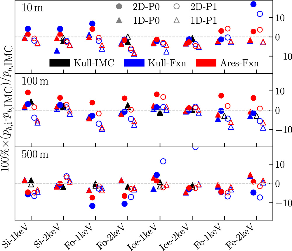
Figure 13. A collection of percent blowoff momentum discrepancies between the IMC and FXN simulations. The colors indicate which code was used to obtain the results. A filled marker indicates that the simulation had zero porosity (P0), while an open marker indicates nonzero porosity (P1), and the shapes correspond to either a full 2D simulation (circles) or an integration of a sweep of 1D simulations (triangles). The porosities used are 62% for SiO2, 69% for Mg2SiO4, 40% for H2O, and 20% for Fe.
Download figure:
Standard image High-resolution imageTable 5. Blowoff Momentum Values and Deflection Velocities for Each Case at 10 μs Using the IMC Simulation
| pb (108 g cm μs−1) ∣ Δv (cm s−1 ) | 10 m | 100 m | 500 m | |||||
|---|---|---|---|---|---|---|---|---|
| Mat. | BB | ρ (g cm−3) | pb | Δv | pb | Δv | pb | Δv |
| SiO2 | 1 keV | 2.65 | 1.76 | 0.723 | 2.39 | 0.981 | 1.29 | 0.530 |
| 1.0 | 1.56 | 1.70 | 2.38 | 2.59 | 1.28 | 1.39 | ||
| 2 keV | 2.65 | 3.52 | 1.45 | 6.74 | 2.77 | 3.30 | 1.35 | |
| 1.0 | 3.00 | 3.26 | 6.04 | 6.57 | 2.94 | 3.20 | ||
| Mg2SiO4 | 1 keV | 3.22 | 1.73 | 0.585 | 2.12 | 0.716 | 1.26 | 0.426 |
| 1.0 | 1.46 | 1.59 | 2.17 | 2.36 | 1.21 | 1.32 | ||
| 2 keV | 3.22 | 3.88 | 1.31 | 6.11 | 2.06 | 2.81 | 0.950 | |
| 1.0 | 3.14 | 3.42 | 5.46 | 5.94 | 2.61 | 2.84 | ||
| H2O | 1 keV | 1.0 | 5.40 | 5.88 | 6.64 | 7.22 | 3.85 | 4.19 |
| 0.6 | 4.84 | 8.78 | 6.10 | 11.1 | 3.49 | 6.33 | ||
| 2 keV | 1.0 | 8.13 | 8.85 | 12.6 | 13.7 | 7.37 | 8.02 | |
| 0.6 | 7.25 | 13.2 | 11.2 | 20.3 | 6.33 | 11.5 | ||
| Fe | 1 keV | 7.877 | 1.77 | 0.244 | 1.65 | 0.228 | 1.08 | 0.149 |
| 6.30 | 1.68 | 0.290 | 1.59 | 0.275 | 1.07 | 0.185 | ||
| 2 keV | 7.877 | 1.95 | 0.269 | 2.42 | 0.334 | 1.53 | 0.211 | |
| 6.30 | 1.85 | 0.319 | 2.32 | 0.401 | 1.51 | 0.261 | ||
Note. At such early times, less than 0.001% of the asteroid's mass has been ejected, so Δv can be calculated using the asteroid's original mass.
Download table as: ASCIITypeset image
Figure 13 depicts how the 2D simulations using the energy deposition model compare to their IMC counterparts. The various markers, colors, and shapes indicate the code used, the simulation method (2D versus 1D integration), and the porosity status. All simulation residuals were compared to results from an IMC simulation. If the 2D IMC simulation for that case failed to reach 10 μs, the comparison was performed at the simulation's end time, which would result in a slightly smaller blowoff momentum discrepancy, but not enough to dominate the distributions (see Section 4.2). Comparisons that utilized the 2D IMC simulation have a black triangle in their data point set, which is the percent deviation between the 1D integration and the full 2D simulation. Cases without the black triangle are instances where the 2D IMC simulation failed to run long enough for a reasonable comparison, and the 1D integration was utilized instead. The standard deviations of the FXN versus IMC residuals shown for each set of 48 simulation comparisons were 6.1%, 3.1%, 4.0%, and 2.9% for the 2D Kull runs, 1D integration Kull runs, 2D Ares runs, and 1D integration Ares runs, respectively. All of the standard deviations are comfortably below the 8.2% estimated discrepancy uncertainty, further demonstrating this model's success.
5.1. Cross-code Comparison
A final argument in favor of this model's validity comes from comparing these results to previously published work. Section 5 of Dearborn et al. (2020) covers a set of simulations that were run in a third mesh-based radiation-hydrodynamics code not utilized in this work. Figure 11 of Dearborn et al. (2020) presents results that are most relevant to this work. This figure contains deflection velocities from a series of 2D simulations with a 560 m, ϕ = 62% SiO2 asteroid using 1, 1.5, and 2 keV BB sources, a 1 Mt yield, and standoff distances at 100 and 500 m. The final deflection velocity values from the simulations were taken at 0.25 ms, substantially longer than 10 μs. The deflection velocity values for each of the relevant BB source points in Dearborn et al.'s (2020) Figure 11 were 1.7, 3.1, 3.8, and 7.6 cm s−1 for the 1 keV/500 m, 1 keV/100 m, 2 keV/500 m, and 2 keV/100 m cases, respectively. Drawing from Table 5, all Δvs from this work are between 80% and 87% of the Dearborn values and still increasing. Therefore, based on these sparse data points, no egregious discrepancy can be inferred.
For further comparison, the scripts used to generate the data points for Dearborn et al. (2020) were procured and used to rerun another set of 48 simulations matching the suite from Section 5 while collecting pb versus time data. Figure 14 represents the pb values at 10 μs collected from the Dearborn suite and compared to the Kull IMC suite using the same methods from Figure 13.

Figure 14. A collection of percent blowoff momentum discrepancies between the IMC and Dearborn simulations. A filled marker indicates that the simulation had zero porosity (P0), while an open marker indicates a nonzero porosity with the same material-percentage combinations from Figure 13 (P1).
Download figure:
Standard image High-resolution imageWhen compared, the percent discrepancy distribution between the Dearborn and Kull IMC suites yielded a standard deviation of 14.5%. It should be emphasized that this study is meant to compare both the Kull IMC results and the closely matched FXN results to another radiation-hydrodynamics code. Though Kull and Ares produce very similar results, there are many likely reasons why the difference between Kull and the Dearborn code is larger. Some potential culprits include utilizing slightly different material models and the lack of a thorough resolution study with the Dearborn code. With more effort, the gap between the two radiation-hydrodynamics codes would mostly likely be bridged with sufficient explanation. However, even the larger percent discrepancy is still much smaller than the uncertainties introduced to the system when all of an asteroid's unknown properties are brought into play.
Finally, Figure 11 of Dearborn et al. (2020) reveals another key detail worthy of examination. Alongside the Δvs for the BB source spectra with a 1 Mt device, the figure also depicts a sweep of simulations at various standoff distances using a "realistic" NED output, which falls between the 1 and 2 keV data points. The writers recommend utilizing this plot when determining which BB source spectrum is best suited for a particular scenario.
6. Conclusion and Future Work
After careful validation and verification against multiple numerical approaches, this nuclear mitigation mission X-ray energy deposition model is complete, accurate, and ready for use in large-scale hydrodynamic simulations. Though the scope of study for this model was significant, eventual extensions are possible. If scenarios with standoff distances of less than 10 m are seriously considered, higher-fluence calculations will be needed to model such cases. In addition, a thorough quantitative study of how mixtures of materials behave when illuminated with NED X-ray radiation will eventually be needed to better connect the generic asteroid-like materials used in this study to more detailed compositional representations for asteroids and comets. This model's largest weakness is a lack of experimental data to compare against; specifically, the detailed response of asteroidal (or surrogate) material to X-rays in the relevant temperature and fluence ranges. A campaign aiming to directly observe material ablated with an X-ray source similar to that of an NED using the University of Rochester OMEGA laser was recently funded via the Federal Yearly Opportunities for Research in Planetary Defense Grant. The team plans to collect data over the next several years. Another, similar proposal using the NIF laser facility at Lawrence Livermore National Laboratory has been formulated, though not yet approved. Should either of these experiments yield data that contradict the simulated results, either a correction or reformulation of this model may be required.
This energy deposition model's completion opens up a vast array of potential studies that can be completed using large-scale hydrodynamic codes. The writers are working to verify that the deposition is working as expected in the hydrocode Spheral (Owen 2014), which can model realistic asteroid shapes and has well-developed strength and damage models that are ideal for late-time simulations. Spheral has been extensively utilized in simulations related to the aforementioned DART mission and has the capability of generating a random rubble-pile distribution that better reflects the actual structure of a rubble-pile asteroid. With successful implementation in Spheral, highly sophisticated simulations are possible that would allow researchers to better simulate the NEO's various structural characteristics. Properties such as the distribution of material/density, rotation, irregular shapes, shadows cast by boulders, the marginal pull of gravity, and even the composition on a larger scale all require more detailed studies of their effect on a mission's outcome. In particular, understanding whether or not an attempted deflection mission will break apart an asteroid has been a long-standing question in the planetary defense community. Utilizing the rubble-pile structure in Spheral with this energy deposition model may eventually allow researchers to do a thorough probe of the deflection/disruption threshold. A better understanding of and reduction in the uncertainties related to the deflection/disruption threshold will provide decision-makers actionable, risk-informed information should a nuclear mitigation be needed to prevent a future impact. Efforts to understand the effects of kinetic impactor and ion-beam deflection mitigation missions will also benefit from NED disruption threshold research.
Should a real planetary defense emergency arise, decisions around launching reconnaissance and/or mitigation missions will need to be informed by state-of-the-art modeling and simulation capabilities. However, fast-running tools that can approximate mitigation outcomes with sufficient accuracy while also supporting integration into mission design optimization studies are a necessary component of preparedness. These faster-running tools must be underpinned by high-fidelity simulations, like the ones described in this paper. Development of an analytical model to determine the necessary yield and standoff distance of an NED for a specific Δv is already underway with the deposition model implemented in Ares. Every detailed, high-fidelity simulation and every broad sensitivity sweep brings the field closer to understanding how effective nuclear mitigation would be. In the event that an Earth-impacting asteroid is located, an operational capability to quickly and credibly assess mission options and uncertainties for planetary defense may potentially save lives and essential infrastructure.
Acknowledgments
The authors would like to thank Doug Miller and the Kull code development team along with Brian Pudliner and the Ares code development team for their extensive assistance over the course of this project. The authors are also grateful to John Michael Owen for motivating the completion of this project, and to Jason Pearl and Kathryn Kumamoto for their steadfast support. This work was performed under the auspices of the U.S. Department of Energy by Lawrence Livermore National Laboratory under contract DE-AC52-07NA27344. LLNL-JRNL-848747.
Appendix A: Model Information
The 1D fit functions depend on the material; the depth in solid material, x = z(1 − ϕ) (cm); the cosine of the angle of incidence,  ; the fluence at the surface, f (kt m−2); the temperature of the source used, T (keV); the length of the source, tend (ns); and the porosity, ϕ.
The deposition function is built out of several different terms. The first term is based on the angle of incidence, the logarithm of the fluence ( ), and the length of the source:
When this function is negative, the deposition is zero.
The remaining functions in the fit depend on the length of the source (tend), the porosity (ϕ), and the fluence corrected for the angle of incidence,

which has units of (kt m−2). The functions use the logarithm of the fluence, F. To handle fluences below the range of our calculations ( ), the logarithm of the fluence is limited to −4, and a scaling function is added to the deposition as follows:
Table 2 describes what these functions model.  is the scaling factor for the overall deposition function:
Here we use exp10 (x) = 10x .
The full deposition function depends on two more terms:


When  , set
, set  and
and  . For materials other than ice at 2 keV, we let
  . Again defining x = z(1 − ϕ) (cm) as the depth in solid material, the full energy deposition function is
Edep is in units of peta erg cm–3.
Appendix B: Prescaled Deposition Function Accuracy
This appendix contains a discussion of the performance of the original suite of raw energy deposition functions before the scaling factor was introduced to correct for discrepancies between FXN and IMC blowoff momenta. A set of surface plots depicting the percent differences between the two 1D suites of 504 simulations for each material/BB combination based on fluence and source duration is shown in Figure 15.

Figure 15. Surface plots depicting the initial blowoff momentum discrepancies in percent between the IMC and function-initiated hydrodynamic suites of 1D simulations with no scaling or adjustments made to the original piecewise energy density functions.
Download figure:
Standard image High-resolution imageThere are multiple trends impacting the accuracy across each variable. Density is a key variable; the X-rays penetrate more deeply into the material to deposit their energy for a low-density material such as ice, so the internal energy reconstruction works well, resulting in good accuracy between IMC and FXN simulations. By contrast, the X-rays cannot penetrate deeply into a high-density material like iron, so all of their energy is concentrated over a smaller region of the surface, which vaporizes and is ejected at high velocity early in the simulation. With such high conversion of energy to kinetic movement early in the iron simulations, the internal energy reconstruction fails by the largest margin. At low fluences, the IMC simulations can take much longer than 100 ns for the reradiated energy fraction to reach convergence compared to high-fluence cases, where by the time selected in Section 3.2, the reradiation has already reached >95% of its final value. When the internal energy time slice is taken, any remaining energy that would eventually be lost to reradiation in IMC simulations is locked into the t = 0 FXN simulation's energy deposition, where reradiation is not possible. This extra energy can artificially inflate the final FXN blowoff momentum values by up to 10%. Finally, the FXN simulations for all materials at higher fluences resulted in less blowoff momentum than the IMC counterparts. Similar to reradiation, when the time slice is taken, there is also kinetic energy from the inward-moving shock wave that is artificially zeroed out, which lowers the total energy of the system and may be partly to blame for the lower pb at high fluences. However, adding the shock-wave kinetic energy back to the system only changed the results by <15%, which was insufficient to offset the discrepancy. Additional trends resulting from the time and temperature dependency of each material's opacity in the IMC simulations are also not matched in the FXN simulations. Such behavior cannot be easily extracted from the IMC simulations and is likely contributing to further discrepancies in the blowoff momentum between the simulation suites.
Various physics-based corrections and adjustments to the energy density profiles to better match the blowoff momentum between the IMC and FXN simulations were explored. However, changes in the materials' thermodynamic properties over the heating process from the source radiation proved to be more complex than simple adjustments could consistently account for. The thermodynamic effects were large enough that even correcting for incomplete reradiation and the shock-wave kinetic energy was insufficient to significantly offset the discrepancy. In order for the energy deposition model development to continue, a scaling factor was added to the baseline, unaltered energy density function to match the final FXN simulation blowoff momentum to the IMC blowoff momentum
Footnotes
- 1
The vast majority of NEOs are asteroids, with a small fraction (0.4%) representing comets (Chodas 2022).
- 2
The radiation fluence from a source decreases with distance according to the inverse square law; the brief flux of radiation that reaches Earth from an NED mission detonated more than 1 million miles away will be less than that of sunlight radiation on a normal day.
- 3
Depending on the device used, between 5% and 10% of the total output energy is released some time after the detonation and is not included in the reported energy yield of a device (Section 1.27 of Glasstone & Dolan 1977).
- 4
A snowplow model allows the material to compress at zero pressure until the porosity is reduced to zero.
- 5
Here, c is the speed of light.
- 6
The 49 parameter sets include six parameters for each of the eight material/BB source combinations plus
 for the Ice-2 keV case.
 - 7
Determined by the residual limits in Figure 15.

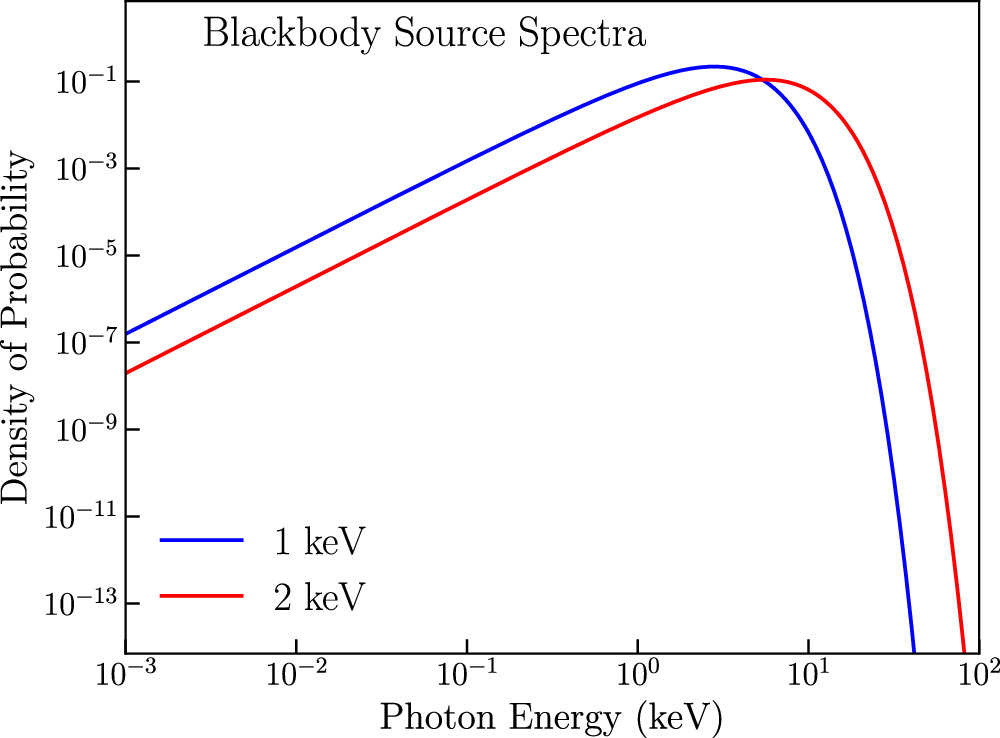
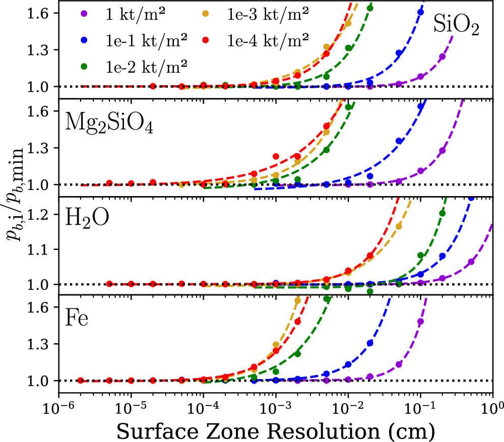
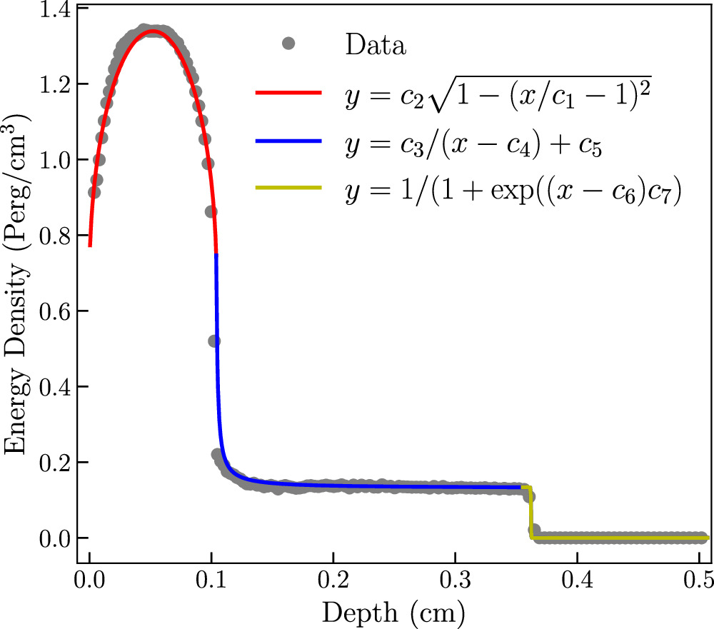
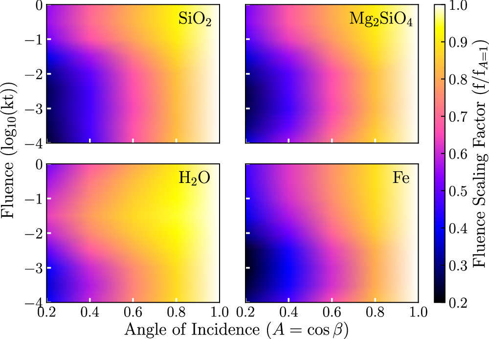
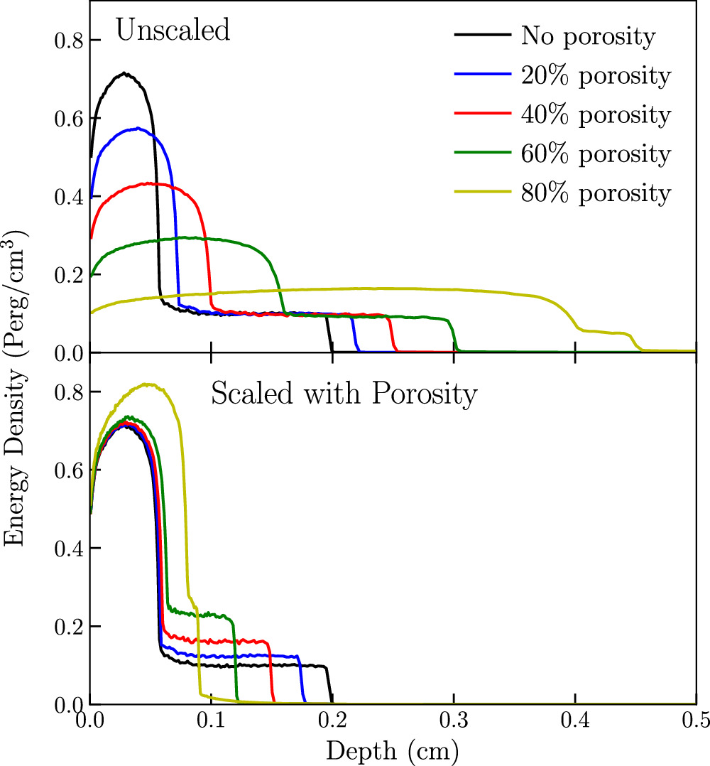
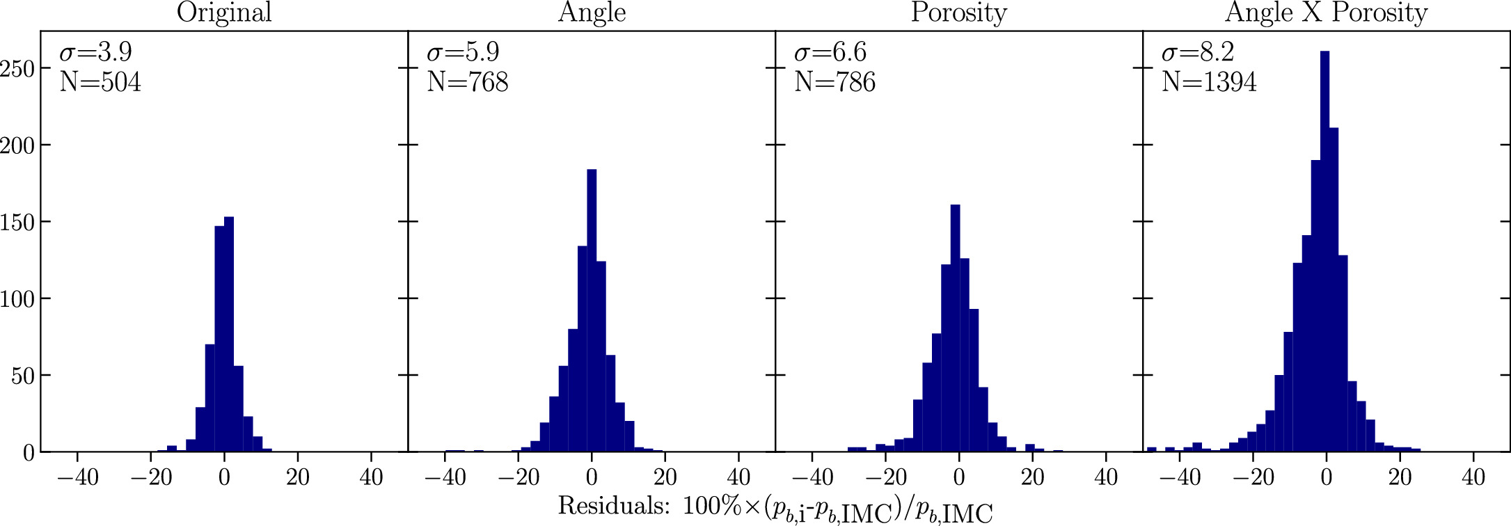